Unlock the Power of MATLAB Transpose: A Simple Guide
MATLAB, a powerful numerical computing environment by MathWorks, offers extensive functionality for matrix manipulations. Understanding linear algebra is crucial for effectively utilizing MATLAB, as many operations rely on its principles. The matlab transpose operation, a fundamental concept, plays a key role in data manipulation and algorithm development. Proficiency in matrix operations like matlab transpose is necessary for engineers, scientists, and researchers using MATLAB for complex calculations.
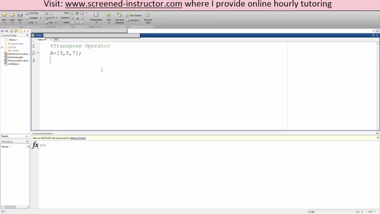
Image taken from the YouTube channel Screened-Instructor , from the video titled MATLAB- Transpose .
MATLAB, short for Matrix Laboratory, stands as a cornerstone in the world of numerical computing and data analysis. Its intuitive interface and powerful toolboxes make it an indispensable resource for engineers, scientists, and researchers across various disciplines.
At the heart of MATLAB's capabilities lies its ability to efficiently manipulate matrices, the fundamental building blocks of many computational tasks. Among the various matrix operations, the transpose stands out as a particularly versatile and essential tool.
The Ubiquitous Transpose: A Cornerstone of Matrix Manipulation
The transpose operation, at its core, involves swapping the rows and columns of a matrix. While seemingly simple, this operation unlocks a surprising range of possibilities in data manipulation, algorithm design, and problem-solving.
Its significance stems from its ability to reorient data, adapt matrices for specific calculations, and provide alternative perspectives on complex datasets.
Why This Guide? Clarity and Practicality in Focus
This guide aims to provide a clear, concise, and practical understanding of the MATLAB transpose function. Whether you're a beginner just starting your journey with MATLAB or an experienced user seeking to deepen your understanding, this resource is tailored to meet your needs.
We will break down the complexities, illustrate with real-world examples, and equip you with the knowledge to confidently wield the power of the transpose in your own MATLAB projects. By the end of this guide, you will not only understand what the transpose does, but also why and how to use it effectively.
Now that we've established MATLAB's core purpose and the transpose's widespread utility, let’s delve into the foundational principles. Understanding what a matrix is, and how its transpose is derived, provides the necessary groundwork for mastering more advanced applications.
Transpose Basics: Matrices and Their Transformations
At its heart, MATLAB revolves around matrices. These rectangular arrays of numbers are fundamental to almost every operation within the environment.
Defining the Matrix
A matrix is, simply put, a rectangular arrangement of numbers, symbols, or expressions organized into rows and columns. Think of it as a table of values.
Each element within the matrix is identified by its row and column index. For example, the element in the second row and third column would be referred to as a2,3.
Matrices are crucial in linear algebra, a branch of mathematics that provides the theoretical underpinning for much of MATLAB's functionality. They are used to represent linear transformations, solve systems of equations, and perform countless other mathematical operations.
In MATLAB, matrices form the bedrock upon which almost all computations are built. Vectors, scalars (single numbers), and even images can be represented and manipulated as matrices.
The Essence of Transpose: Rows Become Columns
The transpose operation is a fundamental transformation applied to matrices. It involves interchanging the rows and columns.
In simpler terms, what was a row in the original matrix becomes a column in the transposed matrix, and vice versa.
If we have a matrix A, its transpose is typically denoted as AT or A'. This simple swap unlocks powerful possibilities in data manipulation and algorithm design.
Visualizing the Transformation: A Concrete Example
To solidify understanding, consider a simple 2x3 matrix:
A = [1 2 3;
     4 5 6]
Applying the transpose operation, we obtain:
A' = [1 4;
      2 5;
      3 6]
Notice how the first row of A (1 2 3) has become the first column of A', and the second row of A (4 5 6) has become the second column of A'.
This visual transformation is key to grasping the core concept of the transpose. It reorients the data, making it suitable for different types of calculations and analyses. The number of rows and columns is also switched when implementing the transpose function. In the A matrix, there are 2 rows and 3 columns. The transposed matrix, A', now has 3 rows and 2 columns.
Now that we've established MATLAB's core purpose and the transpose's widespread utility, let’s delve into the foundational principles. Understanding what a matrix is, and how its transpose is derived, provides the necessary groundwork for mastering more advanced applications.
Vectors: Transposing Row and Column Vectors in MATLAB
Vectors, often perceived as distinct entities, are, in reality, special cases of matrices within the MATLAB environment. Their inherent simplicity allows us to grasp the transpose operation with greater clarity. In this section, we will explore how the transpose operation transforms row vectors into column vectors, and vice versa, with practical examples in MATLAB.
Vectors as Special Matrices
A vector can be visualized as a matrix with either a single row or a single column.
A row vector has dimensions of 1 x n, where 'n' represents the number of elements in the vector.
Conversely, a column vector has dimensions of m x 1, where 'm' is the number of elements.
This matrix representation is crucial because it allows us to apply matrix operations, including the transpose, to vectors seamlessly.
Transposing Row Vectors into Column Vectors
The transpose operation's primary function is to interchange rows and columns. When applied to a row vector, it transforms it into a column vector. Each element, originally arranged horizontally, is now aligned vertically.
Consider a row vector r = [1 2 3].
Its transpose, denoted as r', results in a column vector:
r = [1 2 3];
r_transpose = r'
The output will be:
r_transpose =

     1
     2
     3
This demonstrates the fundamental transformation: the horizontal arrangement becomes vertical.
Transposing Column Vectors into Row Vectors
Conversely, transposing a column vector converts it into a row vector. The vertical arrangement of elements is reoriented horizontally.
Suppose we have a column vector c:
c = [4; 5; 6];
c_transpose = c'
The output will be:
c_transpose =

     4     5     6
Here, the semicolon (;) is used to define a column vector in MATLAB. The transpose operation, c', converts this column vector into its corresponding row vector representation.
Practical MATLAB Examples
Let's solidify our understanding with more MATLAB code examples:
Example 1: Transposing a Row Vector
rowvector = [10 20 30 40];
columnvector = rowvector'; % Transpose using the ' operator
disp(columnvector);
This code snippet first defines a row vector named row
_vector
.Then, it transposes it using the ' operator and assigns the result to column_vector.
Finally, it displays the resulting column vector.
Example 2: Transposing a Column Vector
columnvector = [5; 10; 15; 20];
rowvector = columnvector'; % Transpose using the ' operator
disp(rowvector);
This example mirrors the previous one but starts with a column vector, effectively demonstrating the reverse transformation.
Example 3: Verifying Dimensions After Transpose
vector = [1 2 3 4 5];
sizebefore = size(vector);
transposedvector = vector';
sizeafter = size(transposedvector);

disp(['Size before transpose: ' num2str(sizebefore)]);
disp(['Size after transpose: ' num2str(sizeafter)]);
This example checks and displays the dimensions of the vector before and after transposition, further illustrating the change in orientation.
These examples highlight how easily MATLAB handles vector transposition, solidifying the concept through practical application. The transpose operation provides the flexibility needed for various data manipulations and algorithm implementations.
Complex Conjugate Transpose: Handling Complex Numbers in MATLAB
Having explored the transposition of real-valued vectors and matrices, it's time to address a critical aspect of MATLAB: its handling of complex numbers. MATLAB's default transpose operation isn't just a simple row-column swap; it also performs a conjugation when dealing with complex numbers. Understanding this behavior is paramount for accurate and efficient computation.
Understanding Complex Numbers in MATLAB
Complex numbers, essential in various fields such as electrical engineering and quantum mechanics, consist of a real part and an imaginary part. They are represented in the form a + bi, where a is the real part, b is the imaginary part, and i is the imaginary unit (√-1).
MATLAB seamlessly supports complex numbers. You can directly define a complex number using the i or j notation.
For example:
z = 3 + 4i;
Here, z is a complex number with a real part of 3 and an imaginary part of 4.
MATLAB provides built-in functions like real(z) and imag(z) to extract the real and imaginary components of a complex number, respectively.
The Conjugate Transpose: Default Behavior
In MATLAB, the default transpose operator (') performs a complex conjugate transpose. This means that when applied to a matrix containing complex numbers, it not only swaps the rows and columns but also takes the complex conjugate of each element.
The complex conjugate of a complex number a + bi is a - bi. In other words, the sign of the imaginary part is flipped.
For example, the complex conjugate of 3 + 4i is 3 - 4i.
Therefore, for a complex matrix A, the element in the i-th row and j-th column of A' is the complex conjugate of the element in the j-th row and i-th column of A.
Illustrative Examples: Conjugate Transpose in Action
Let's examine how the conjugate transpose affects a complex matrix in MATLAB:
A = [1+i, 2-i; 3, 4+2i];
A_transpose = A'
In this example, A is a 2x2 complex matrix. Applying the transpose operator results in A_transpose:
A_transpose =
1.0000 - 1.0000i   3.0000
2.0000 + 1.0000i   4.0000 - 2.0000i
Notice that the rows and columns have been swapped, and the imaginary parts of each element have had their signs flipped.
Let's consider another example to solidify understanding:
B = [i, 1; 2, -i]
B_transpose = B'
The output will be:
B_transpose =

        0 - 1.0000i   2.0000
        1.0000             0 + 1.0000i
This example further illustrates the combined effect of transposition and complex conjugation.
Understanding the conjugate transpose is critical when dealing with complex matrices, as it directly impacts calculations in areas such as signal processing and quantum mechanics. In the subsequent section, we'll explore situations where you might want to avoid conjugation and use a simple, non-conjugate transpose.
Non-Conjugate Transpose: The .' Operator
We've seen how the default transpose operator in MATLAB (') performs a complex conjugate transpose, which is a useful and often desired behavior. However, there are situations where you only want to swap the rows and columns of a matrix without conjugating the complex elements. This is where the non-conjugate transpose operator (.') comes into play.
Understanding the Non-Conjugate Transpose
The non-conjugate transpose operator (.') in MATLAB provides a way to transpose a matrix without affecting the imaginary parts of its complex elements.
It performs a simple row-column swap, leaving the complex numbers untouched.
This is crucial when dealing with algorithms or mathematical operations that rely on the precise values of complex numbers and where conjugation would introduce errors or inconsistencies.
Differentiating Between ' and .'
The key distinction lies in how these operators handle complex numbers.
The default transpose (') performs both transposition and complex conjugation.
The non-conjugate transpose (.') performs only transposition. It's vital to internalize this difference to avoid unexpected results, especially when working with complex matrices.
When to Use the .' Operator: Practical Examples
Avoiding Unintended Conjugation
Consider a scenario where you're working with a matrix representing a quantum mechanical system. The complex elements might represent probability amplitudes.
Conjugating these amplitudes would fundamentally alter the system's state and lead to incorrect results. In such cases, using the .' operator is essential to maintain the integrity of the data.
Preserving Complex Data
Let's illustrate with a simple example:
A = [1+2i, 3+4i; 5+6i, 7+8i]; % A complex matrix
B = A.'; % Non-conjugate transpose
C = A';  % Conjugate transpose
disp(B);
disp(C);
In this example, B will be [1+2i, 5+6i; 3+4i, 7+8i], while C will be [1-2i, 5-6i; 3-4i, 7-8i]. Notice how B preserves the original imaginary components.
Signal Processing Applications
The .' operator is invaluable in signal processing, particularly when dealing with Fourier transforms or other frequency-domain representations.
Operations like calculating the correlation or convolution of complex signals often require transposition without conjugation to maintain the correct phase relationships.
Using the conjugate transpose in these situations would lead to incorrect signal analysis.
In conclusion, the non-conjugate transpose operator (.') is a vital tool in MATLAB for scenarios where you need to transpose matrices containing complex numbers without altering their imaginary components. Understanding the difference between '.' and ' is crucial for accurate and reliable computation in various scientific and engineering applications.
Transposing Multi-Dimensional Arrays in MATLAB
Having explored the intricacies of transposing matrices and vectors, including the nuances of complex conjugate and non-conjugate transposes, it's natural to extend our understanding to arrays with higher dimensionality. MATLAB's capabilities extend far beyond two-dimensional matrices, allowing for the creation and manipulation of multi-dimensional arrays.
This section will explore how the transpose operation behaves when applied to these higher-dimensional structures, providing a more complete perspective on its functionality within MATLAB.
Creating Multi-Dimensional Arrays
In MATLAB, multi-dimensional arrays are extensions of matrices, where each element is identified by more than two indices. Think of them as arrays of matrices.
These arrays can be created using functions like zeros, ones, rand, or by concatenating existing arrays along different dimensions using cat.
For example, to create a 3x3x3 array of zeros, you would use the command: A = zeros(3, 3, 3);. This creates a three-dimensional array where each "slice" is a 3x3 matrix.
Understanding Dimension Ordering
Before delving into transposition, it’s crucial to understand how MATLAB orders the dimensions of a multi-dimensional array. The first dimension corresponds to the rows, the second to the columns, the third to the "depth," and so on.
This ordering is essential for predicting how the transpose function will rearrange the array's elements.
The Default Transpose and Dimension Swapping
The default transpose function in MATLAB, denoted by the single quote ('), swaps the first two dimensions of an array.
For a matrix, this is simply the familiar row-column swap.
However, for a multi-dimensional array, the effect is a re-orientation of the array, where the order of the first two dimensions is reversed.
For example, consider a 2x3x4 array A. Applying A' will result in a 3x2x4 array. The rows and columns (the first two dimensions) have been interchanged, while the third dimension remains unchanged.
Practical Examples
Let's solidify this with a concrete example. Suppose we have a 2x3x2 array A:
A = cat(3, [1 2 3; 4 5 6], [7 8 9; 10 11 12])
This creates a 2x3x2 array. If we apply the transpose operation:
B = A'
The resulting array B will be of size 3x2x2. The rows and columns have been swapped.
To verify, consider element A(1,2,1) which equals 2. After transposition, this element is now located at B(2,1,1).
This example highlights the core principle: the default transpose swaps only the first two dimensions, leaving the remaining dimensions in their original order.
Beyond the Default: Custom Dimension Permutations
While the default transpose swaps only the first two dimensions, MATLAB offers the permute function for more complex dimension rearrangements.
The permute function allows you to specify a new order for all the dimensions of an array. For example, to swap the first and third dimensions of an array A, you could use:
B = permute(A, [3 2 1]);
Here, [3 2 1] indicates that the original third dimension becomes the first, the second remains the second, and the original first dimension becomes the third. The permute function offers the flexibility to tailor the dimension ordering to specific needs.
Non-Conjugate Transpose and Multi-Dimensional Arrays
The non-conjugate transpose operator (.) also applies to multi-dimensional arrays, behaving similarly to its operation on matrices.
It swaps the first two dimensions without performing complex conjugation, ensuring that the imaginary parts of complex elements remain unchanged.
This is especially important when working with multi-dimensional arrays containing complex data, where preserving the integrity of the complex values is crucial.
Having explored the intricacies of transposing matrices and vectors, including the nuances of complex conjugate and non-conjugate transposes, it's natural to extend our understanding to arrays with higher dimensionality. MATLAB's capabilities extend far beyond two-dimensional matrices, allowing for the creation and manipulation of multi-dimensional arrays.
This section will explore how the transpose operation behaves when applied to these higher-dimensional structures, providing a more complete perspective on its functionality within MATLAB.
Practical Applications of the Transpose Operation
The transpose operation in MATLAB isn't just a theoretical exercise; it's a powerful tool with applications across diverse fields. From reshaping data for analysis to manipulating signals and images, understanding transpose unlocks a range of possibilities. Let's delve into some real-world scenarios where this operation proves indispensable.
Data Manipulation and Reshaping
One of the most common uses of the transpose operation is in data manipulation. Often, data is collected or stored in a format that isn't ideal for analysis or computation. The transpose function allows us to easily reshape data to fit the required format.
For example, consider a scenario where you have data representing measurements taken over time, stored in rows. To perform certain statistical analyses or machine learning algorithms, you might need to have each measurement type represented in columns instead.
% Sample data: Measurements over time (rows)
data = [1 2 3; 4 5 6; 7 8 9];

% Transpose the data to have measurements in columns
transposed_data = data';
% Display the transposed data
disp(transposed_data);
In this simple example, the transpose operation effortlessly converts the data from a row-oriented to a column-oriented format, making it suitable for further processing.
Signal Processing: Filtering and Convolution
In signal processing, the transpose operation frequently arises in the context of filter design and convolution. Filters are often represented as row vectors, and to apply them to a signal (another vector), we might need to transpose the filter vector to perform matrix multiplication or convolution operations correctly.
% Sample signal
signal = [1 2 3 4 5];

% Filter coefficients (row vector)
filter_coeffs = [0.2 0.3 0.5];
% Transpose the filter coefficients for convolution
transposed_filter = filter_coeffs';
% Perform convolution (example)
filtered_signal = conv(signal, filter_coeffs);
% Display the filtered signal
disp(filtered_signal);
Transposing the filter coefficients ensures that the convolution operation is performed as intended, yielding the desired filtered signal. The transpose operation ensures compatibility in dimensions for signal processing algorithms.
Image Processing: Rotating and Reflecting Images
The transpose operation can also be applied in image processing to achieve certain effects. While MATLAB provides dedicated functions for image rotation and reflection, understanding how transpose affects image data can be insightful.
An image can be represented as a matrix, where each element corresponds to the pixel intensity. Transposing this matrix essentially swaps the rows and columns, which can be interpreted as a reflection of the image across the main diagonal.
% Sample image data (grayscale)
image_data = [10 20 30; 40 50 60; 70 80 90];
% Transpose the image data
transposed_image = image_data';
% Display the transposed image data
disp(transposed_image);
While this isn't a typical image rotation, it demonstrates how matrix manipulation, including transpose, can influence image representation. More complex image transformations often rely on matrix operations that build upon this fundamental understanding.
Machine Learning: Feature Matrix Manipulation
In machine learning, the transpose operation plays a crucial role in preparing data for model training. Feature matrices, which represent the input data for machine learning algorithms, often need to be transposed to align with the expected input format of the algorithms.
For instance, if you have data where each row represents a sample and each column represents a feature, some algorithms might require the data to be organized with samples in columns and features in rows.
% Sample feature matrix (rows = samples, columns = features)
feature_matrix = [1 2 3; 4 5 6; 7 8 9];
% Transpose the feature matrix
transposed_featurematrix = featurematrix';

% Display the transposed feature matrix
disp(transposedfeaturematrix);
The transpose operation provides a quick and efficient way to reorient the feature matrix, ensuring compatibility with the chosen machine learning algorithm. This is crucial for ensuring the algorithm processes data as intended.
Beyond the Examples: A Versatile Tool
These examples represent just a fraction of the applications where the transpose operation proves useful. Its ability to reshape data, facilitate matrix operations, and prepare data for various algorithms makes it an indispensable tool in the MATLAB programmer's arsenal. By mastering this fundamental operation, you'll unlock a wide range of possibilities for solving real-world problems in various domains.
Having explored the practical applications of the transpose operation, it’s equally crucial to discuss potential pitfalls and best practices. A solid understanding of common errors and how to avoid them will significantly improve the reliability and efficiency of your MATLAB code.
Best Practices, Common Errors, and Troubleshooting
Mastering the transpose operation in MATLAB requires more than just knowing how to use the ' or .' operators. It involves understanding potential errors, optimizing performance, and developing sound coding habits. This section provides a guide to avoiding common mistakes and adopting best practices for using transpose effectively.
Common Errors and Pitfalls
Several common errors can arise when working with the transpose operation in MATLAB. Awareness of these issues is the first step in preventing them.
Dimension Mismatches
Perhaps the most frequent error is encountering dimension mismatches. This occurs when the dimensions of a matrix or array do not align with the expected input of a subsequent operation.
For instance, attempting to add a 3x2 matrix to the transpose of a 3x2 matrix will result in an error because the transpose will be 2x3.
Always double-check the dimensions of your matrices and arrays before and after applying the transpose operator. Use the size() function to verify dimensions programmatically.
Incorrect Usage with Complex Numbers
When dealing with complex numbers, understanding the difference between the conjugate transpose (') and the non-conjugate transpose (.') is paramount.
Using the conjugate transpose when you intend to only transpose can lead to unexpected results due to the conjugation of imaginary components.
Carefully consider whether conjugation is desired. If not, consistently use the .' operator for non-conjugate transpose.
Forgetting Order of Operations
In complex expressions, the order of operations involving the transpose can be easily overlooked, leading to unintended consequences.
Parentheses can be your best friend here. Explicitly define the order of operations to ensure that the transpose is applied at the correct stage of the calculation.
Overwriting Data
Be mindful when transposing matrices or arrays and assigning the result back to the original variable. This overwrites the initial data.
If the original data is needed later, create a new variable to store the transposed result.
Tips and Recommendations for Avoiding Errors
Preventing errors requires a proactive approach. Here are some practical tips for ensuring the correct and efficient use of the transpose operation.
Verifying Dimensions
Always use the size() function to check the dimensions of your matrices and arrays, especially before performing operations that depend on specific dimensions. This helps catch dimension mismatches early.
You can use assertions in your code to automatically check for expected sizes and raise an error if they are not met.
Using Comments
Add comments to your code to clarify the purpose of each transpose operation. This is particularly helpful when dealing with complex operations or when the intent is not immediately obvious.
Good comments make your code easier to understand and debug.
Testing and Debugging
Thoroughly test your code with various inputs, including edge cases and complex numbers. Use MATLAB's debugging tools to step through your code and inspect the values of variables at each step.
Write unit tests to verify the correctness of your code.
Leverage Functions
When performing transpose operations repeatedly, encapsulate the logic within a function. This promotes code reusability and reduces the likelihood of errors.
Functions also make your code more modular and easier to maintain.
Optimizing Code Performance with Transpose
While correctness is paramount, optimizing code performance is also crucial, especially when dealing with large datasets.
Avoiding Unnecessary Transposes
Minimize the number of transpose operations in your code. Each transpose takes time, and unnecessary operations can significantly slow down your code.
Carefully consider whether a transpose is truly needed or if the same result can be achieved with a different approach.
Pre-allocation
If you know the size of the transposed matrix or array in advance, pre-allocate memory for it using functions like zeros() or ones(). This can improve performance by avoiding dynamic memory allocation during the transpose operation.
Vectorization
MATLAB is highly optimized for vectorized operations. Whenever possible, use vectorized operations instead of loops to perform calculations involving transposed matrices or arrays.
Vectorization can significantly improve the speed of your code.
Importance of Dimensional Awareness
In conclusion, mastering the transpose operation in MATLAB goes hand in hand with meticulous attention to dimensions.
Understanding the impact of transpose on matrix and array sizes, distinguishing between conjugate and non-conjugate transposes, and adopting proactive error-prevention strategies are key to writing robust and efficient MATLAB code. By incorporating these best practices, you can confidently leverage the power of transpose in your numerical computations.
Video: Unlock the Power of MATLAB Transpose: A Simple Guide

FAQ: Mastering MATLAB Transpose Operations
Here are some common questions about using the transpose operator in MATLAB. We'll clarify its function and usage for efficient matrix manipulation.
What does the MATLAB transpose operator actually do?
The MATLAB transpose operator (') switches the rows and columns of a matrix. This means that the element in the i-th row and j-th column becomes the element in the j-th row and i-th column. Essentially, it flips the matrix over its main diagonal. It is a core element for working with the matlab transpose.
How is the complex conjugate transpose different from a simple transpose?
In MATLAB, the single quote (') performs a complex conjugate transpose. This not only transposes the matrix but also takes the complex conjugate of each element. For purely real matrices, this is the same as a regular transpose. Use .' for a non-conjugate matlab transpose when dealing with complex numbers.
Can I transpose a non-square matrix in MATLAB?
Yes, MATLAB allows you to transpose non-square matrices. The resulting matrix will have dimensions swapped. For example, transposing a 2x3 matrix will result in a 3x2 matrix. The principles of matlab transpose remain the same.
What happens if I try to transpose a scalar value in MATLAB?
Transposing a scalar value (a single number) in MATLAB simply returns the same value. The matlab transpose operation has no effect because a scalar is considered a 1x1 matrix, and swapping its row and column doesn't change it.