Standard Curve Secrets: Ace Your Analysis Now!

Accuracy in quantitative analysis relies heavily on the standard curve. Laboratories worldwide, including those adhering to ISO 17025 standards, utilize it as a cornerstone for precise measurements. The concept of linearity, a critical attribute of the standard curve, ensures proportional relationships between analyte concentration and instrument response. Successful implementation using software like GraphPad Prism enhances data reliability.

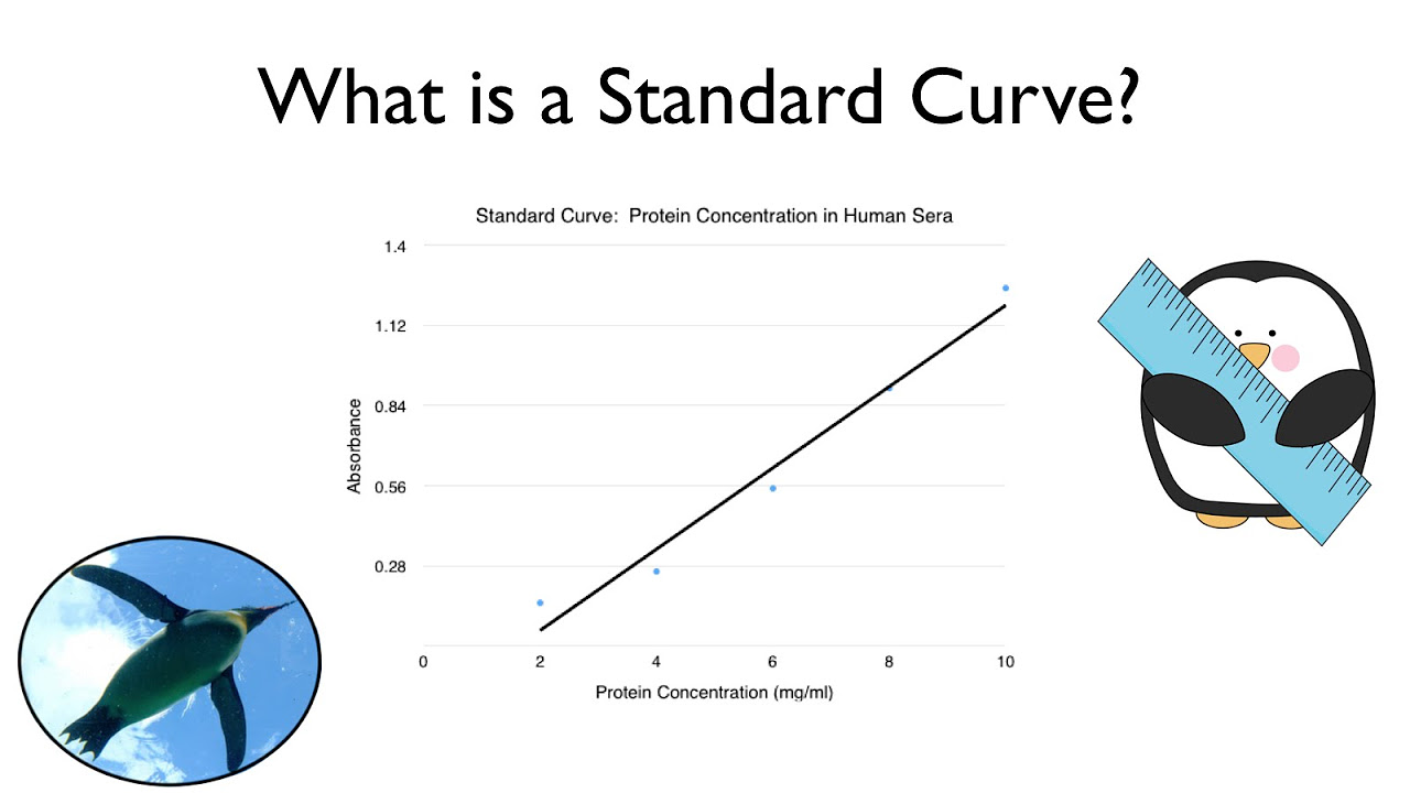
Image taken from the YouTube channel ThePenguinProf , from the video titled What is a Standard Curve? .

In the realm of quantitative analysis, where precision and accuracy are paramount, the standard curve stands as an indispensable tool. It acts as a bridge, connecting measured signals to corresponding concentrations, enabling researchers and analysts to transform raw data into meaningful, quantifiable insights.

The Cornerstone of Quantitative Analysis

The standard curve isn't merely a graph; it's the foundation upon which quantitative measurements are built. Whether determining the concentration of a drug in a patient's blood, quantifying pollutants in environmental samples, or measuring enzyme activity in a biochemical assay, the standard curve plays a pivotal role.

It provides the necessary framework to interpret instrument readings and derive reliable concentration values. Without a properly constructed and validated standard curve, the results of any quantitative analysis are inherently questionable.

Calibration: Ensuring Reliability and Trustworthiness

Calibration is the linchpin of any analytical process. It establishes the relationship between the instrument's response and the known concentration of an analyte. Accurate calibration, achieved through the use of carefully prepared standards, is essential for generating reliable results.

A poorly calibrated instrument, or a flawed standard curve, will inevitably lead to inaccurate quantitation, potentially compromising the validity of research findings, clinical diagnoses, or regulatory compliance. The consequences of inaccurate results can be far-reaching.

They can impact critical decisions in various fields, including healthcare, environmental protection, and product development.

Mastering Standard Curves: A Path to Enhanced Data Quality

Mastering the art and science of standard curves requires a comprehensive understanding of the underlying principles, meticulous attention to detail in experimental procedures, and a rigorous approach to data analysis and validation. Key strategies for achieving mastery include:

• Careful Standard Preparation: Ensuring the purity, stability, and accurate concentration of standards is crucial.

• Optimized Experimental Design: Selecting an appropriate concentration range, minimizing experimental errors, and employing proper controls are vital.

• Rigorous Data Analysis: Choosing the right regression model, identifying and addressing outliers, and validating the curve's performance are essential.

• Continuous Monitoring and Improvement: Regularly assessing the standard curve's performance, troubleshooting any issues, and implementing best practices are necessary for long-term reliability.

By embracing these strategies, analysts can unlock the full potential of standard curves, elevate the quality of their data, and enhance the reliability of their analytical results, leading to more informed decisions and greater confidence in their findings.

The consequences of inaccurate results can be far-reaching. They can impact critical decisions in various fields, including healthcare, environmental protection, and product development. Therefore, before delving into the practical aspects of building and evaluating standard curves, it's crucial to first establish a solid understanding of the fundamental principles that govern their function.

Understanding the Foundation: Standard Curve Principles Explained

At its core, a standard curve is a graphical representation of the relationship between the signal generated by an analytical instrument and the corresponding concentration of a known substance, the analyte, that you wish to measure. This graph serves as a calibration tool, enabling the determination of unknown analyte concentrations by comparing their signals to those of the standards. The principle is straightforward: the higher the concentration of the analyte, the stronger the signal.

Deconstructing the Standard Curve

A standard curve is not a monolithic entity, but rather a carefully constructed assembly of essential components working in concert. Understanding these components is key to grasping how standard curves function.

• Standards: These are solutions of known concentrations of the analyte.

  They are the backbone of the standard curve, providing the reference points against which unknown samples are measured.

• Samples: These are the unknown solutions containing the analyte whose concentration you want to determine.

  The signal from these samples is compared to the standard curve to extrapolate the concentration.

• Measurements: These are the instrument readings (e.g., absorbance, fluorescence, peak area) obtained for both the standards and the samples.

  These readings must be accurate and precise to ensure the reliability of the standard curve.

The process begins with the preparation of a series of standards, typically at varying concentrations that span the expected range of the unknown samples. Each standard is then analyzed using the chosen instrument, and the resulting signal is recorded. These data points (concentration vs. signal) are plotted on a graph, creating the standard curve. When an unknown sample is analyzed, its signal is located on the curve, and the corresponding concentration is determined by interpolation.

Linearity: The Key to Accurate Quantitation

The accuracy of a standard curve hinges on its linearity, which refers to the degree to which the signal is directly proportional to the concentration of the analyte. Ideally, a standard curve should exhibit a linear relationship over a defined concentration range.

Within this linear range, a change in concentration will produce a predictable and proportional change in signal, allowing for accurate quantitation.

• Why is Linearity Important?

  Non-linear regions of the standard curve can lead to inaccurate concentration determinations, as the relationship between signal and concentration becomes complex and unpredictable.

• Identifying and Addressing Non-Linearity:

  It's essential to identify the linear range of the standard curve and restrict quantitation to this region. In some cases, non-linear data may be fit with a non-linear regression model, but this approach requires careful consideration and validation.

By ensuring that the standard curve is linear within the range of interest, researchers can confidently translate instrument readings into accurate and reliable concentration values, forming a solid foundation for quantitative analysis.

The principles underlying standard curves give them their power. With the groundwork now established, it’s time to translate these concepts into practice. The next critical step involves constructing a standard curve that not only looks good on paper but also delivers trustworthy results.

Building a Better Standard Curve: Key Factors for Success

Constructing a reliable standard curve is more than just plotting data points; it's a meticulous process demanding attention to detail and adherence to best practices. The accuracy of your downstream analysis hinges directly on the quality of the standard curve you create. Therefore, understanding and implementing key factors for success is paramount.

The Foundation: Preparing Accurate Standards

At the heart of every reliable standard curve lies the accuracy of the standards themselves. If the standards are flawed, the entire curve, and consequently all subsequent measurements, will be compromised.

Emphasizing Proper Preparation

Standards should always be prepared using high-purity materials and calibrated equipment. Pay close attention to the manufacturer’s instructions for any reference material. Use appropriate solvents and diluents. Minimize sources of contamination.

Mastering Serial Dilutions

Serial dilutions are a common technique for creating a range of standard concentrations. However, they are also a potential source of error. Each dilution step amplifies any inaccuracies introduced earlier. To minimize this, use calibrated pipettes, mix thoroughly after each dilution, and consider performing dilutions in triplicate to assess precision.

A best practice is to prepare fresh standards each time you run an assay. If that is not possible, meticulously document storage conditions and expiration dates. Properly stored standards are crucial to maintaining their integrity and the accuracy of your standard curve.

Achieving Optimal Linearity: Choosing the Right Concentration Range

Linearity is a critical characteristic of a standard curve. It signifies a direct, proportional relationship between the analyte concentration and the signal it produces. A linear curve simplifies data analysis and ensures that you can accurately extrapolate concentrations of unknown samples.

Factors Influencing Linearity

The linear range of a standard curve depends on both the assay being used and the instrument used to measure the signal. Operating outside the instrument's linear range or exceeding the detection capabilities of the assay will lead to non-linear results.

Strategies for Selecting the Optimal Range

• Start with a broad range of concentrations during initial experiments to identify the region of linearity.

• Then, narrow the range to focus on the concentrations relevant to your samples.

• Ensure the selected range adequately covers the expected concentrations of your unknown samples while remaining within the linear portion of the curve.

• Consider performing a linearity study to objectively assess the range over which the assay is linear.

Minimizing Errors and Variability: Enhancing the Quality of Your Curve

Even with carefully prepared standards and an optimized concentration range, experimental errors can still creep in and affect the quality of your standard curve. By minimizing these errors, you can improve the precision and reliability of your results.

Addressing Potential Sources of Error

• Pipetting errors: Use calibrated pipettes and practice proper pipetting techniques.
• Temperature fluctuations: Maintain a stable temperature during the assay.
• Instrument drift: Regularly calibrate the instrument and monitor its performance.
• Reagent instability: Use fresh reagents and follow recommended storage conditions.
• Matrix effects: Consider the potential impact of the sample matrix on the assay and implement appropriate controls.

The Importance of Replication

Performing measurements in triplicate or even higher replicates can help reduce the impact of random errors. Averaging multiple measurements provides a more accurate estimate of the true signal, leading to a more precise standard curve. Replicates allow you to identify and exclude outliers.

Documentation is Key. Thoroughly document every step of the standard curve construction process, including the source and purity of standards, dilution procedures, instrument settings, and any deviations from the protocol. This documentation is essential for troubleshooting and ensuring the reproducibility of your results.

The principles underlying standard curves give them their power. With the groundwork now established, it’s time to translate these concepts into practice. The next critical step involves constructing a standard curve that not only looks good on paper but also delivers trustworthy results.

Evaluating Standard Curve Performance: Metrics That Matter

Once a standard curve is constructed, the work isn't over. Rigorous evaluation is essential to ensure that the curve meets the required standards for reliability and accuracy. Several key metrics allow us to scrutinize a standard curve's performance and determine its suitability for quantitative analysis.

Understanding the R-squared Value (R²)

The R-squared value, often referred to as the coefficient of determination, is a statistical measure that represents the proportion of the variance in the dependent variable (signal) that is predictable from the independent variable (concentration).

In simpler terms, it indicates how well the data points fit the regression line. An R² value closer to 1 suggests a strong correlation, meaning that the model explains a large proportion of the variability in the response data.

However, it's crucial to understand that a high R² value alone does not guarantee a good standard curve. It merely indicates a strong statistical relationship. Other factors, such as accuracy and precision, must also be considered. A commonly accepted R² threshold is 0.99 or higher, but this may vary depending on the specific application and regulatory requirements.

Assessing Accuracy and Precision

Accuracy refers to how close a measurement is to the true or accepted value. In the context of a standard curve, it reflects how well the curve predicts the known concentrations of the standards. Accuracy can be assessed by calculating the percent recovery of the standards.

Precision, on the other hand, refers to the repeatability or reproducibility of a measurement. A precise standard curve will yield similar results when the same sample is measured multiple times. Precision is typically evaluated by calculating the coefficient of variation (CV) or relative standard deviation (RSD) of replicate measurements.

Both accuracy and precision are vital for a reliable standard curve. A curve can be precise but inaccurate (consistently off-target) or accurate but imprecise (yielding highly variable results). The ideal standard curve is both accurate and precise.

Determining the Limits of Detection (LOD) and Quantitation (LOQ)

The Limit of Detection (LOD) is the lowest concentration of an analyte that can be reliably detected, but not necessarily quantified, by a given analytical procedure. It represents the point at which the signal is significantly different from the background noise.

The Limit of Quantitation (LOQ) is the lowest concentration of an analyte that can be quantitatively determined with acceptable precision and accuracy. The LOQ is always higher than the LOD.

Understanding and utilizing LOD and LOQ are critical for determining the usable range of the standard curve. Results below the LOD should be considered non-detectable, while results between the LOD and LOQ should be interpreted with caution. Only results above the LOQ can be reliably quantified.

Calculation Methods for LOD and LOQ

Various methods exist for calculating LOD and LOQ, including:

• Signal-to-Noise Ratio: LOD is often estimated as 3 times the standard deviation of the blank signal divided by the slope of the standard curve, while LOQ is estimated as 10 times the same value.
• Standard Deviation of the Response: LOD and LOQ can also be calculated based on the standard deviation of the response and the slope of the calibration curve.
• Calibration Curve Method: This method involves using the standard deviation of the y-intercepts of the calibration curves.

The choice of method depends on the specific analytical procedure and the available data.

The Role of Quality Control (QC) Samples

Quality Control (QC) samples are samples with known concentrations of the analyte that are run alongside the unknown samples to monitor the performance of the standard curve and the entire analytical process. QC samples should be prepared independently from the standards used to construct the standard curve.

By analyzing QC samples at different concentrations within the curve's range, you can assess the accuracy and precision of the standard curve and identify potential problems, such as drift or matrix effects.

QC samples are an indispensable tool for validating the reliability of your results. If QC sample results fall outside of acceptable limits, the entire batch of samples should be re-analyzed.

The insights gained from a meticulously constructed standard curve are only as valuable as the analysis and interpretation applied to the data. It's one thing to generate a curve; it's quite another to extract meaningful information that drives accurate and reliable conclusions. This section provides a detailed guide to navigating the data analysis process, focusing on regression analysis, sample concentration calculations, and outlier management to ensure the integrity of your results.

Data Analysis and Interpretation: Extracting Meaningful Insights

Regression Analysis: Selecting the Right Model

Regression analysis is the cornerstone of transforming raw data from a standard curve into usable information. It allows us to establish the mathematical relationship between the signal (absorbance, fluorescence, etc.) and the known concentrations of our standards.

The choice of regression model is critical, and it depends on the observed relationship between concentration and signal.

Linear Regression

For many assays, a simple linear regression model is sufficient, assuming that the signal increases linearly with concentration across the range tested.

This model is represented by the equation: y = mx + b, where 'y' is the signal, 'x' is the concentration, 'm' is the slope, and 'b' is the y-intercept.

Non-Linear Regression

However, standard curves often exhibit non-linear behavior, particularly at higher concentrations. In these cases, non-linear regression models are more appropriate.

Quadratic, cubic, or logarithmic models may provide a better fit for the data.

Selecting the most appropriate model can be guided by statistical criteria such as minimizing the residual sum of squares or maximizing the adjusted R-squared value. Visual inspection of the data and the regression line is also essential to confirm that the model accurately reflects the observed relationship.

Calculating Unknown Sample Concentrations

Once the regression model is established, it's time to determine the concentrations of your unknown samples. This is achieved by measuring the signal of each sample and using the regression equation to extrapolate the corresponding concentration.

Interpolation

The process involves interpolation, where the sample signal is located on the standard curve, and the corresponding concentration is read off.

For linear regression, this is straightforward: rearrange the equation (x = (y - b) / m) to solve for 'x', the concentration, using the sample's signal ('y').

For non-linear models, the calculation may require more complex mathematical operations or the use of specialized software.

Dilution Factors

It is crucial to account for any dilution factors applied to the samples during preparation. Remember to multiply the calculated concentration by the dilution factor to obtain the actual concentration in the original sample.

Identifying and Addressing Outliers

Outliers are data points that deviate significantly from the expected trend and can disproportionately influence the regression analysis and subsequent concentration calculations. Identifying and addressing outliers is essential for ensuring data integrity.

Grubbs' Test

Statistical tests such as Grubbs' test or Dixon's Q-test can be used to objectively identify potential outliers. These tests assess whether a data point is significantly different from the rest of the data set.

Justification for Removal

However, removing outliers should not be done arbitrarily. There should be a justifiable reason for excluding a data point, such as a known experimental error, a sample handling issue, or instrument malfunction. All removed data points and the reasons for their removal must be documented transparently.

Re-Analysis

If an outlier is removed, it is important to re-analyze the data and reconstruct the standard curve. Assess whether the removal of the outlier significantly improves the accuracy and reliability of the curve.

Alternative Approaches

If no clear justification for removing an outlier exists, consider using robust regression methods that are less sensitive to outliers, or explore alternative regression models that may better accommodate the data.

Troubleshooting Common Standard Curve Challenges

The insights gained from a meticulously constructed standard curve are only as valuable as the analysis and interpretation applied to the data. It's one thing to generate a curve; it's quite another to extract meaningful information that drives accurate and reliable conclusions. This section provides a detailed guide to navigating the data analysis process, focusing on regression analysis, sample concentration calculations, and outlier management to ensure the integrity of your results.

Even with meticulous planning and execution, standard curves can sometimes present challenges. Poor linearity, high variability, and unexpected results are common hurdles that can compromise the accuracy and reliability of your data. This section provides a practical guide to troubleshooting these issues, offering insights into their root causes and providing actionable solutions to get your standard curves back on track.

Addressing Poor Linearity

Poor linearity is a frequent problem, indicating that the relationship between concentration and signal deviates significantly from a straight line. This deviation invalidates the assumptions of linear regression and compromises the accuracy of concentration estimates.

Potential Causes of Non-Linearity

Several factors can contribute to poor linearity:

• Exceeding the dynamic range of the assay: At high concentrations, the signal may plateau due to saturation of the detection system.

• Inadequate standard preparation: Errors in serial dilutions or improper mixing can lead to inaccurate standard concentrations.

• Matrix effects: Components in the sample matrix may interfere with the signal, particularly at higher concentrations.

• Instrument malfunction: A malfunctioning detector or light source can introduce non-linearity.

Strategies for Improving Linearity

• Optimize the concentration range: Narrow the concentration range to focus on the linear portion of the curve. Consider using lower concentrations if saturation is suspected.

• Refine standard preparation: Use calibrated pipettes and ensure thorough mixing at each dilution step. Prepare fresh standards for each experiment.

• Address matrix effects: Use appropriate blanks and consider matrix matching by adding the sample matrix to the standards.

• Verify instrument performance: Regularly calibrate and maintain the instrument according to the manufacturer's recommendations.

• Consider non-linear regression: If linearity cannot be achieved, explore non-linear regression models such as quadratic or sigmoidal fits, if justified by the data.

Mitigating High Variability

High variability, manifested as large error bars or poor reproducibility, reduces the precision of your measurements and makes it difficult to draw meaningful conclusions.

Sources of Variability

• Pipetting errors: Inconsistent pipetting is a major source of variability, particularly in serial dilutions.

• Temperature fluctuations: Temperature variations can affect reaction rates and signal intensity.

• Inconsistent incubation times: Variations in incubation times can lead to inconsistent signal development.

• Reader inconsistencies: Plate readers may have well-to-well or run-to-run variability.

Strategies for Reducing Variability

• Improve pipetting technique: Use calibrated pipettes, practice proper pipetting techniques, and consider using multi-channel pipettes for serial dilutions.

• Maintain temperature control: Perform assays in a temperature-controlled environment, such as a water bath or incubator.

• Standardize incubation times: Use timers and ensure consistent incubation times for all samples.

• Optimize plate reader settings: Ensure proper mixing before reading, read plates from the same orientation each time, and use appropriate filters.

• Increase the number of replicates: Increasing the number of replicates can reduce the impact of random errors.

Investigating Unexpected Results

Unexpected results, such as concentrations that are significantly higher or lower than expected, can indicate underlying problems with the assay or samples.

Root Cause Analysis

• Sample contamination: Contamination can introduce interfering substances or alter the concentration of the analyte.

• Matrix interference: As previously mentioned, matrix effects can skew results.

• Reagent degradation: Expired or improperly stored reagents can lead to inaccurate results.

• Calculation errors: Errors in data analysis or calculations can lead to incorrect concentration estimates.

Corrective Actions

• Repeat the assay with fresh samples and reagents: This helps rule out contamination or reagent degradation.

• Evaluate the impact of the matrix: Perform recovery experiments by spiking known amounts of the analyte into the sample matrix to assess matrix effects.

• Verify calculations: Double-check all calculations and data analysis steps.

• Consult the assay protocol: Review the assay protocol for any potential deviations or troubleshooting tips.

• Seek expert advice: If the problem persists, consult with experienced colleagues or the assay manufacturer for assistance.

By systematically addressing these common standard curve challenges, you can improve the accuracy, precision, and reliability of your quantitative analyses, ensuring that your data is sound and your conclusions are well-supported.

Best Practices for Long-Term Reliability of Standard Curves

After navigating the initial hurdles and achieving a well-performing standard curve, the focus shifts to maintaining its reliability over time. The longevity of a standard curve's accuracy is paramount for consistent, dependable results. This section outlines crucial best practices to ensure your standard curves remain robust and trustworthy for the long haul.

The Cornerstone: Regular Instrument Calibration

Regular instrument calibration is the bedrock of long-term reliability. Analytical instruments are complex systems that can drift out of specification due to wear, environmental factors, or component aging. If your analytical instruments are not properly calibrated, it will result in innacurate standard curves.

Why Calibration Matters

Calibration involves comparing an instrument's output to a known standard and adjusting it to minimize deviations. This process ensures that measurements remain accurate and consistent over time, directly impacting the integrity of standard curves.

Neglecting regular calibration can lead to systematic errors that invalidate previous and future analyses.

Establishing a Calibration Schedule

Develop a calibration schedule based on the instrument manufacturer's recommendations, the frequency of use, and the criticality of the measurements.

More frequent calibrations may be necessary for instruments used in high-throughput or critical applications.

Maintain detailed records of all calibration activities, including dates, standards used, and any adjustments made.

Preserving Integrity: Standard Storage and Handling

The integrity of your standards is just as vital as instrument calibration. Standards are the reference points upon which the entire standard curve is built; compromised standards lead to flawed results.

Optimal Storage Conditions

Store standards under conditions that prevent degradation. This typically involves:

• Controlled temperatures (often refrigeration or freezing).
• Protection from light.
• Use of appropriate storage containers (e.g., amber vials for light-sensitive compounds).

Follow the manufacturer's guidelines for storage, but be prepared to adapt them based on your specific laboratory environment and compounds.

Minimizing Contamination and Degradation

Avoid repeated freeze-thaw cycles, which can degrade many standards. Aliquot standards into smaller volumes to minimize the need for repeated thawing.

Use calibrated pipettes and volumetric glassware to ensure accurate dilutions. Prepare fresh working standards regularly, as stock solutions can degrade over time.

The Power of Documentation: Traceability and Quality Assurance

Comprehensive documentation is not just a regulatory requirement; it's a critical element of long-term reliability. Detailed records provide a clear audit trail, enabling you to identify and address potential issues that may arise.

Essential Documentation Practices

Maintain meticulous records of:

• Standard preparation (including source, lot number, and preparation date).
• Instrument parameters.
• Raw data.
• Data analysis steps.
• Any deviations from established protocols.

Implement a system for tracking samples and standards throughout the entire analytical process.

Ensuring Traceability and Auditability

All data and procedures should be traceable to the analyst who performed them. This accountability helps ensure that best practices are followed and errors are promptly identified.

Regularly review documentation to identify trends or potential problems that may affect the reliability of your standard curves.

By diligently adhering to these best practices – prioritizing regular instrument calibration, ensuring proper standard storage and handling, and maintaining comprehensive documentation – you can safeguard the long-term reliability of your standard curves and the accuracy of your analytical results.

Video: Standard Curve Secrets: Ace Your Analysis Now!

Play Video