Joint Relative Frequency Explained: The Ultimate Guide!
Joint relative frequency, a crucial tool in data analysis, helps reveal relationships between variables. The application of contingency tables, a method heavily utilized by statisticians, facilitates the calculation of joint relative frequency. Furthermore, understanding the output from software like SPSS is essential for interpreting these calculations, providing insightful data-driven conclusions and market research.
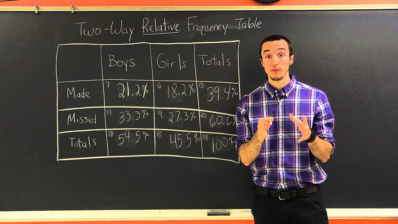
Image taken from the YouTube channel Milanese Math , from the video titled Joint, Marginal, and Conditional Relative Frequency | Milanese Math Tutorials .
Joint Relative Frequency (JRF) is a statistical measure that reveals the proportion of observations that possess a specific combination of characteristics from two or more categorical variables. It's a crucial tool for understanding the interplay between these variables within a dataset.
Defining Joint Relative Frequency
At its core, Joint Relative Frequency represents the ratio of the number of times a specific combination of categories occurs to the total number of observations.
Imagine a scenario where we analyze customer data, looking at both their preferred product type and their geographic location. JRF would tell us the proportion of customers who prefer a specific product and live in a specific region, relative to the entire customer base.
This allows us to move beyond simply looking at individual variables and to explore their relationships. The formula is simple:
JRF = (Frequency of Specific Combination) / (Total Number of Observations)
Significance in Probability and Statistics
JRF plays a vital role in probability and statistics by providing insights into dependencies between categorical variables. It forms the basis for more advanced statistical analyses, such as chi-square tests and measures of association.
By calculating and analyzing JRF, we can determine whether certain combinations of categories occur more or less frequently than would be expected by chance. This can reveal meaningful relationships that might be hidden when analyzing variables in isolation.
For instance, JRF can help determine if there's a statistically significant association between a particular treatment and patient outcomes in a clinical trial. Or, if a specific marketing campaign is more effective in certain demographic groups.
Leveraging JRF for Data Analysis Insights
Data analysis utilizes JRF to extract actionable insights from datasets. By quantifying the relationships between categorical variables, we can identify patterns, trends, and potential areas for improvement.
JRF helps us understand the "why" behind the numbers. It allows us to move beyond simple descriptions of data and to explore the underlying factors that drive observed outcomes.
For example, a retailer could use JRF to analyze sales data and identify which product categories are most popular in different regions. This insight could then inform decisions about product placement, marketing campaigns, and inventory management.
Real-World Applications of JRF
The applications of Joint Relative Frequency span a wide range of fields:
- Market Research: Identifying customer segments based on demographics and purchasing behavior.
- Healthcare: Analyzing relationships between risk factors and disease prevalence.
- Education: Examining the correlation between student demographics and academic performance.
- Social Sciences: Investigating the association between socioeconomic factors and political attitudes.
- Business Analytics: Understanding the interplay between marketing strategies and customer engagement.
In each of these applications, JRF provides a powerful tool for uncovering hidden relationships and making data-driven decisions. By understanding how variables interact, we can gain a deeper understanding of the world around us and make more informed choices.
Joint Relative Frequency provides a powerful lens through which to examine the interplay between categorical variables. Before we can fully appreciate its applications and nuances, however, it's essential to understand the fundamental concepts that underpin its calculation and interpretation: frequency distributions and the organization of data sets. These are the building blocks upon which JRF is constructed.
Foundational Concepts: Frequency Distributions and Data Sets
Frequency Distributions: The Stepping Stone to JRF
A frequency distribution is a tabular or graphical representation that summarizes the occurrences of different values within a dataset. It provides a clear picture of how data is distributed across various categories or intervals.
Think of it as a tally of each unique outcome in a series of observations. For example, if we surveyed 100 people about their favorite color, a frequency distribution would show how many people chose each color option (red, blue, green, etc.).
This is the precursor to JRF.
Without understanding the frequency of individual categories, we cannot begin to analyze the joint occurrences of combinations of categories that JRF reveals. Frequency distributions provide the raw material for JRF calculations.
Building a Frequency Distribution
Constructing a frequency distribution involves several key steps:
- Identify the unique values or categories within the variable being analyzed.
- Tally the number of times each value or category appears in the dataset.
- Present the tallies in a table or graph, showing the frequency of each value.
For instance, you might create a frequency distribution showing the number of customers who purchased each type of product from your online store during a specific period.
Data Sets: The Foundation for JRF Calculations
A data set is a collection of related data, typically organized in a structured format. It's the raw material from which we derive insights, including Joint Relative Frequencies.
Data sets often take the form of tables, spreadsheets, or databases, with rows representing individual observations and columns representing variables or attributes.
To calculate JRF, data sets must contain categorical variables. These variables represent characteristics or qualities that can be divided into distinct categories, such as gender, product type, or geographic region.
Organizing Data for JRF
The organization of a data set is crucial for efficient JRF calculation. Each row should represent a single observation, and each column should represent a variable.
For JRF, you'll need at least two categorical variables in your dataset. The goal is to analyze the relationship between these variables, and that requires having them clearly defined and organized.
Consider a data set of customer information, with columns for "Product Purchased" (categorical) and "Region" (categorical). This would be ideal for calculating the JRF of customers who bought a specific product in a specific region.
Data Cleaning and Preparation
Before performing JRF calculations, it's essential to clean and prepare the data. This may involve:
- Handling missing values: Deciding how to deal with incomplete data points.
- Correcting errors: Identifying and fixing inaccuracies in the data.
- Ensuring consistency: Standardizing the format and coding of categorical variables.
The Interplay of Probability and JRF
Probability is the measure of the likelihood that an event will occur. JRF is intrinsically linked to probability because it estimates the probability of a specific combination of events occurring.
When we calculate the JRF of customers who prefer "Product A" and live in "Region B," we are essentially estimating the probability that a randomly selected customer will both prefer "Product A" and live in "Region B."
JRF as an Empirical Probability
JRF can be interpreted as an empirical probability, meaning it is based on observed data rather than theoretical assumptions. The more data we have, the more accurate our estimate of the probability becomes.
For instance, if we analyzed a small sample of customers, our JRF might be significantly different from the true probability for the entire customer base. With a larger, more representative sample, the JRF provides a more reliable estimate.
Conditional Probability and JRF
JRF also lays the foundation for understanding conditional probability, which is the probability of an event occurring given that another event has already occurred.
By analyzing JRFs, we can begin to explore how the probability of one event changes depending on the occurrence of another event. This sets the stage for more advanced statistical analyses that examine relationships between variables.
Mastering Two-Way Tables (Contingency Tables)
With a solid grasp of frequency distributions as the groundwork, we can now transition to the central tool for understanding Joint Relative Frequency: the two-way table, also known as a contingency table. This table provides a structured way to visualize and analyze the relationship between two categorical variables, offering a clear path to calculating and interpreting JRF.
Two-Way Tables: Visualizing Joint Relative Frequency
A two-way table is essentially a grid that displays the frequencies of observations based on two categorical variables. It provides a clear visual representation of how these variables intersect and allows us to easily calculate Joint Relative Frequencies. Think of it as a roadmap that guides you through the relationships within your data.
The rows of the table typically represent the categories of one variable, while the columns represent the categories of the second variable. The cells at the intersection of rows and columns contain the frequencies, indicating the number of observations that fall into both categories.
Constructing a Two-Way Table: A Step-by-Step Guide
Creating a two-way table involves a systematic process:
-
Identify the Two Categorical Variables: The first step is to clearly define the two variables you want to analyze. These variables should be categorical, meaning they represent distinct categories or groups.
-
Determine the Categories for Each Variable: Next, identify all possible categories for each variable. These categories will form the rows and columns of your table. Ensure the categories are mutually exclusive and collectively exhaustive.
-
Tally the Frequencies: Go through your dataset and count how many observations fall into each combination of categories. This is the core of the process.
For example, count how many observations belong to category A of variable 1 and category B of variable 2.
-
Populate the Table: Enter the tallies into the corresponding cells of the table. Each cell will now display the frequency of observations for that specific combination of categories.
-
Calculate Row and Column Totals (Marginal Frequencies): Sum the frequencies in each row to obtain the row totals (marginal frequencies). Do the same for each column. These totals will be useful for calculating relative frequencies later.
-
Calculate the Grand Total: Sum all the frequencies in the table (or sum the row totals or column totals) to obtain the grand total. This represents the total number of observations in your dataset.
Example: Building a Two-Way Table
Let's say we want to analyze the relationship between gender (Male/Female) and preferred mode of transportation (Car/Bus/Train).
Our two-way table would look something like this:
| Car | Bus | Train | Total | |
|---|---|---|---|---|
| Male | ||||
| Female | ||||
| Total |
We would then go through our dataset and tally the number of males who prefer cars, males who prefer buses, and so on, filling in the corresponding cells.
Calculating Joint Relative Frequency within the Table
Once the two-way table is constructed, calculating Joint Relative Frequency becomes straightforward. The formula is:
Joint Relative Frequency = (Frequency of the cell) / (Grand Total)
In essence, you're dividing the number of observations in a specific category combination by the total number of observations. This gives you the proportion of observations that belong to that particular combination.
Finding JRF: Illustrative Examples
Using our previous example, let's say the completed two-way table looks like this:
| Car | Bus | Train | Total | |
|---|---|---|---|---|
| Male | 30 | 15 | 5 | 50 |
| Female | 20 | 20 | 10 | 50 |
| Total | 50 | 35 | 15 | 100 |
To find the Joint Relative Frequency of "Male and Car," we would divide the frequency of that cell (30) by the grand total (100):
JRF (Male and Car) = 30 / 100 = 0.3 or 30%
This means that 30% of the total observations are males who prefer cars.
Similarly, the JRF for "Female and Train" would be:
JRF (Female and Train) = 10 / 100 = 0.1 or 10%
This indicates that 10% of the total observations are females who prefer trains.
By calculating the Joint Relative Frequency for each cell in the two-way table, you can gain a comprehensive understanding of the relationships between the two categorical variables. This understanding is crucial for making informed decisions and drawing meaningful insights from your data.
Related Frequency Types: Marginal and Conditional Relative Frequency
Having dissected the structure and application of Joint Relative Frequency, it's crucial to understand its relationship with other types of frequencies that offer unique, yet interconnected, perspectives on the same dataset. Specifically, we will now explore Marginal and Conditional Relative Frequencies, clarifying their distinctions from JRF and demonstrating how each contributes to a more comprehensive data analysis.
Differentiating Marginal Relative Frequency from Joint Relative Frequency
Marginal Relative Frequency examines the distribution of a single variable, disregarding the influence of the other variable present in the two-way table. It focuses on the totals along the margins of the table (hence the name "marginal"), representing the proportion of observations that fall into each category of that single variable.
In contrast, Joint Relative Frequency focuses on the intersection of two variables, indicating the proportion of observations that belong to specific combinations of categories from both variables. While JRF drills down to specific pairings, Marginal Relative Frequency takes a broader, more aggregated view.
Imagine analyzing customer preferences for coffee type (e.g., espresso, latte) and milk choice (e.g., almond, oat). The JRF would tell you the proportion of customers who prefer espresso with almond milk. The Marginal Relative Frequency, on the other hand, would tell you the overall proportion of customers who prefer espresso, irrespective of their milk choice.
The formula for Marginal Relative Frequency is quite simple:
Marginal Relative Frequency (Variable A) = (Total Frequency of Category in A) / (Grand Total of All Frequencies)
It's important to note that Marginal Relative Frequencies can be calculated for each category within each variable, providing a clear picture of the overall distribution of individual variables.
Understanding Conditional Relative Frequency and its Connection to JRF
Conditional Relative Frequency explores the probability of an event occurring given that another event has already occurred. It hones in on a specific subset of the data, allowing for analysis of relationships within particular conditions.
This contrasts with JRF, which considers the joint occurrence of two events relative to the entire dataset. Conditional Relative Frequency focuses on the probability of one event given another, while JRF focuses on the probability of both events occurring together.
The link between Conditional Relative Frequency and JRF lies in their mathematical relationship. Conditional Relative Frequency is calculated by dividing the Joint Relative Frequency of two events by the Marginal Relative Frequency of the condition event.
Conditional Relative Frequency (A given B) = JRF (A and B) / Marginal Relative Frequency (B)
This formula highlights that Conditional Relative Frequency utilizes JRF as a component in its calculation, building upon the foundation laid by understanding the joint probabilities.
Examples: Distinct Perspectives on Data
To illustrate the unique perspectives offered by each frequency type, consider a study examining the relationship between exercise habits (regular or irregular) and the occurrence of heart disease (yes or no).
- Joint Relative Frequency: Might reveal that 5% of the population both exercises regularly and does not have heart disease.
- Marginal Relative Frequency: Might show that 40% of the population exercises regularly, regardless of whether they have heart disease.
- Conditional Relative Frequency: Could demonstrate that among those who exercise regularly, only 2% have heart disease. This provides critical insights into the impact of exercise on heart disease.
Each of these percentages offers a different piece of the puzzle.
JRF paints a picture of co-occurrence, Marginal Relative Frequency describes individual variable distributions, and Conditional Relative Frequency illuminates relationships within specific subsets. By considering all three, a more nuanced and complete understanding of the data emerges.
Having explored the mechanics of calculating Joint Relative Frequency and its relationship to other frequency types, it's time to shift our focus to its tangible applications. Understanding where and how JRF is used transforms it from an abstract concept into a powerful analytical tool.
Practical Applications of Joint Relative Frequency
Joint Relative Frequency finds its utility across diverse fields, offering nuanced insights into relationships between categorical variables. From unraveling consumer behavior to optimizing healthcare strategies, JRF provides a robust framework for data-driven decision-making.
Decoding Real-World Scenarios with JRF
The beauty of JRF lies in its adaptability. Consider these real-world applications:
- Market Research: Understanding customer preferences by analyzing relationships between product type and demographic factors. For instance, what proportion of millennials prefer eco-friendly packaging?
- Healthcare: Investigating the correlation between treatment type and patient outcome, revealing the effectiveness of different interventions for specific patient groups.
- Education: Examining the connection between teaching methods and student performance, identifying strategies that yield the best results for various student demographics.
- Risk Assessment: In finance, JRF can assess the joint probability of different adverse events occurring, aiding in the development of robust risk management strategies.
- Manufacturing: Analyzing the relationship between production processes and defect rates, pinpointing areas for improvement in quality control.
In essence, JRF can be applied whenever you seek to understand how two categorical variables interact within a population.
Interpreting JRF Results Through Data Analysis
Calculating JRF is only the first step. The real value emerges from interpreting the results using established data analysis techniques.
Several approaches can enhance your analysis:
- Comparative Analysis: Compare JRF values across different categories to identify significant relationships. For instance, is the JRF for "Treatment A and Positive Outcome" significantly higher than "Treatment B and Positive Outcome?"
- Visualization: Represent JRF data visually using heatmaps or clustered bar charts to quickly identify patterns and outliers. Visualizations can make complex relationships more accessible and understandable.
- Statistical Significance Testing: Employ statistical tests, such as the Chi-square test, to determine if the observed relationships are statistically significant or simply due to random chance.
- Segmentation: Use JRF to segment your data into distinct groups based on shared characteristics, allowing for targeted interventions or strategies.
By combining JRF with these techniques, you can extract meaningful insights and translate data into actionable strategies.
Understanding Variable Interactions Through JRF
JRF provides a lens for understanding how variables interact, revealing dependencies and associations that might otherwise go unnoticed. Consider these perspectives:
- Positive Correlation: A high JRF value for a specific combination of categories indicates a positive association between those categories. For example, a high JRF for "Exercise Regularly and Lower Blood Pressure" suggests a positive correlation.
- Negative Correlation: A low JRF value, relative to other combinations, suggests a negative association or independence between the categories.
- Causation vs. Correlation: It's crucial to remember that JRF reveals correlations, not necessarily causation. Further investigation is often needed to establish causal relationships.
- Confounding Variables: Be aware of potential confounding variables that might influence the observed relationships. Consider factors that may be affecting both variables under study.
By carefully examining JRF values and considering potential confounding factors, you can gain a deeper understanding of the complex interplay between variables.
Industry-Specific Examples of JRF in Action
Let's examine specific examples to illustrate the practical utility of JRF:
Market Research
A market research firm uses JRF to analyze customer survey data. They create a two-way table showing the relationship between age group (e.g., 18-24, 25-34) and preferred social media platform (e.g., Instagram, TikTok).
By calculating the JRF, they determine the proportion of 18-24 year olds who prefer TikTok. This insight informs targeted advertising campaigns and content strategies. A high JRF value would indicate a strong preference, justifying increased investment in TikTok marketing for that demographic.
Healthcare
A hospital analyzes patient data to assess the effectiveness of different treatment protocols for pneumonia. They create a two-way table showing the relationship between treatment type (e.g., Antibiotic A, Antibiotic B) and patient outcome (e.g., Recovered, Not Recovered).
The JRF reveals the proportion of patients treated with Antibiotic A who recovered. Comparing this JRF to that of Antibiotic B helps the hospital identify the more effective treatment for its patient population. This data helps hospitals determine optimal treatment strategies.
These examples highlight the power of JRF to transform raw data into actionable intelligence, enabling organizations to make more informed decisions and achieve better outcomes.
Having explored the mechanics of calculating Joint Relative Frequency and its relationship to other frequency types, it's time to shift our focus to its tangible applications. Understanding where and how JRF is used transforms it from an abstract concept into a powerful analytical tool.
Examples and Case Studies: JRF in Action
To truly grasp the power of Joint Relative Frequency, it's crucial to examine it in action. This section delves into specific examples and case studies, illustrating how JRF is calculated, interpreted, and utilized across diverse domains. We'll also address potential pitfalls, such as limitations and biases, offering strategies for critical interpretation.
Deconstructing JRF Through Concrete Examples
Let's start with a straightforward example to solidify the process of JRF calculation and interpretation.
Imagine a survey conducted at a local library, examining the relationship between age group and preferred book genre. The data collected is summarized in a two-way table.
| Fiction | Non-Fiction | Total | |
|---|---|---|---|
| Under 30 | 80 | 20 | 100 |
| 30-50 | 60 | 40 | 100 |
| Over 50 | 40 | 60 | 100 |
| Total | 180 | 120 | 300 |
To calculate the JRF for "Under 30 and Fiction," we divide the number of respondents under 30 who prefer fiction (80) by the total number of respondents (300). The JRF is therefore 80/300 = 0.267 or 26.7%.
This signifies that 26.7% of all library survey respondents are under 30 and prefer fiction.
Similarly, the JRF for "Over 50 and Non-Fiction" is 60/300 = 0.20 or 20%.
This reveals that 20% of all respondents are over 50 and prefer non-fiction.
By calculating and comparing these JRF values, we can gain insights into the relationship between age and book genre preference within the surveyed population.
JRF in Action: Unveiling Insights Through Case Studies
Beyond simple examples, JRF proves invaluable in complex real-world scenarios. Here are a few case studies highlighting its practical application.
Market Research: Targeted Advertising Campaigns
A marketing firm wants to optimize its advertising campaigns for a new product. They conduct a survey to analyze the relationship between customer income level (Low, Medium, High) and their likelihood of purchasing the product (Yes, No).
Using JRF, they can identify which income groups are most likely to purchase the product.
For example, if the JRF for "High Income and Yes" is significantly higher than other combinations, the firm can focus its advertising efforts on high-income demographics, leading to a more effective and cost-efficient campaign.
Healthcare: Evaluating Treatment Effectiveness
A hospital is evaluating the effectiveness of two different treatments for a specific disease (Treatment A, Treatment B). They track patient outcomes (Improved, No Improvement) for each treatment group.
By calculating the JRF between treatment type and patient outcome, they can determine which treatment is more effective.
A higher JRF for "Treatment A and Improved" compared to "Treatment B and Improved" would suggest that Treatment A is more effective in improving patient outcomes for that disease.
Education: Identifying Effective Teaching Methods
A school district wants to identify the most effective teaching methods (Method 1, Method 2) for improving student performance on standardized tests (Pass, Fail).
By analyzing the JRF between teaching method and student performance, the district can determine which method leads to higher pass rates.
If the JRF for "Method 1 and Pass" is higher, it suggests that Method 1 is more effective in helping students pass the standardized tests.
Navigating the Limitations and Biases in JRF Analysis
While JRF is a powerful tool, it's essential to acknowledge its limitations and potential biases.
One key limitation is that JRF only reveals association, not causation. Just because two variables are jointly frequent doesn't mean one causes the other.
There might be confounding variables influencing the relationship.
Furthermore, the data used to calculate JRF might be biased.
For example, if the survey sample is not representative of the population, the resulting JRF values might not accurately reflect the true relationships.
Another potential bias arises from sample size. Small sample sizes can lead to unstable JRF estimates that don't generalize well to the broader population.
Mitigating Bias and Interpreting Results Critically
To mitigate bias and ensure reliable interpretations, consider the following strategies:
- Ensure Representative Sampling: Strive to collect data from a sample that accurately reflects the population of interest. Use random sampling techniques whenever possible.
- Consider Confounding Variables: Be aware of potential confounding variables that might be influencing the observed relationships. Collect data on these variables and incorporate them into the analysis.
- Use Adequate Sample Sizes: Ensure that the sample size is large enough to provide stable and reliable JRF estimates. Conduct power analysis to determine the appropriate sample size.
- Interpret with Caution: Avoid drawing causal conclusions based solely on JRF analysis. Acknowledge the limitations of the analysis and consider alternative explanations for the observed relationships.
- Cross-Validate Findings: Whenever possible, cross-validate the JRF findings with other data sources or analytical techniques. This can help to confirm the robustness of the results.
By being aware of these limitations and biases and implementing appropriate mitigation strategies, you can use JRF to gain valuable insights from your data while avoiding potentially misleading conclusions. Critical interpretation is key to leveraging the full potential of JRF in data analysis.
Video: Joint Relative Frequency Explained: The Ultimate Guide!

Frequently Asked Questions: Joint Relative Frequency
Here are some frequently asked questions about joint relative frequency to help you better understand the concept and its applications.
What exactly is joint relative frequency?
Joint relative frequency represents the proportion of times a specific combination of categories occurs within a dataset. It's calculated by dividing the frequency of that combination by the total number of observations. This gives you a relative frequency for a specific "joint" occurrence.
How is joint relative frequency different from marginal relative frequency?
Joint relative frequency considers two (or more) variables simultaneously, showing the proportion of observations that fall into specific categories for both variables. Marginal relative frequency, on the other hand, looks at the distribution of one variable at a time, ignoring the other variables.
Where would I typically use joint relative frequency?
You'd commonly use joint relative frequency in contingency tables or two-way tables. These tables display the frequency of different combinations of two categorical variables. Analyzing the joint relative frequencies within the table helps reveal relationships or associations between those variables.
Why is joint relative frequency useful?
Understanding joint relative frequencies allows you to identify patterns and dependencies between different categories. For instance, you could analyze customer data to see the joint relative frequency of customers who bought product A and product B, helping you tailor marketing strategies accordingly.